Setting Up a Reconstruction

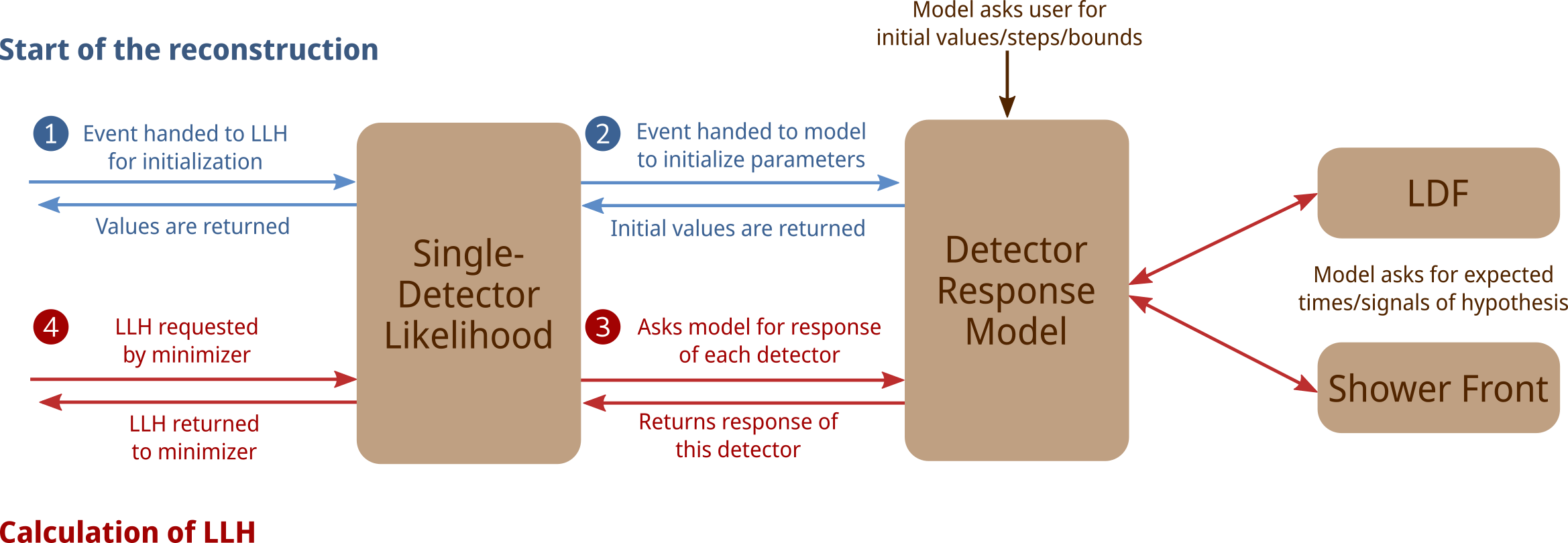
There are several main items that need to be linked to set up a reconstruction. The pieces generally follow this information flow scheme.

This page describes the relevant steps for setting up all of the pieces to being your own reconstruction chain. Examples are given below that detail what the typical parameters that must be set are/do. However, since each detector has its own specific needs and characteristics, other parameters may have to be set. For more, see rock_bottom/resources/examples and rock_bottom/python/segments.

LDF Construction

For a given reconstrucion, a lateral distribution function (LDF) must be chosen. This could either describe the way that the signal amplitudes are distributed w.r.t. the shower axis or that of the arrival times. For more on the LDFs, see Particle distribution functions or Radio-emission distribution functions.

The LDFs all have their own pybindings and can easily be reconstructed using, e.g.

from icecube import rock_bottom
loglog = rock_bottom.ldf.LogLog() # initialize a log-log parabola particle LDF
plane = rock_bottom.showerfront.TimePlane() # initialize a plane arrival-front LDF

For more examples and further functionality, see rock_bottom/resources/test/test_ldfs.py.

Signal Model Construction

The signal model knows about the average signals that are generated using the LDF that was constructed previously. Below is a pseudo example of the construction of a signal model

from icecube import rock_bottom

tray.AddService("LaputopSignalModel", "LaputopSignalAmplitudeModel",
    LDF = loglog, # the model needs to know about the ldf
    ParameterNames   = RbList([RbPair("slopeLdf", 0) , RbPair("slopeLdf", 1)]),
    ParameterValues  = [       2.6,                    0.30264],
    BoundNames       = RbList([RbPair("slopeLdf", 0) , RbPair("lgSref", 0)]),
    BoundValues      = [       (1.9, 3.1),             (-3., 8.)],
    StepNames        = RbList([RbPair("slopeLdf", 0) , RbPair("lgSref", 0)]),
    StepValues       = [       0.6,                    1.],
    )

Note the extra parameters that are passed such as ParameterNames and ParameterNames. These parameters define the phase space that will be searched during the minimization. The name of the parameter is is always give with a RbPair. Internally, which parameters are being used in a reconstruction are dynamically found during runtime. They must link with what is expected by the LDFs. For instance, the log-log LDF expects three parameters to be defined, two which define the slope (slopeLdf) and one which defines the overall amplitude (lgSref). In this example, the slope parameters are being defined to be initialized with values 2.6 and 0.30264 (note that these two parameters correspond to the “beta” and “gamma” of the log-log LDF).

The BoundNames and BoundValues define the range of allowed values that the minimizer is allowed to explore. The first slope parameter (RbPair("slopeLdf", 0) AKA “beta”) is allowed to be between 1.9 and 3.1, while the other slope parameter has no defined bound. Note that the default value for the bounds is +/- inf. The normalization term (RbPair("lgSref", 0) AKA S125) is fixed to be between -3 and 8.

The StepNames and StepValues correspond to how quickly the minimizer will step through phase space. These values should be approximately (order of magnitude) how far you think your initialization is from the true answer. MINUIT (the underlying minimizer) dynamically changes the step size during run time, so no need for this to be perfect. The first slope parameters (RbPair("slopeLdf", 0) AKA “beta”) has a step size of 0.6 while the second slope parameter has no defined step size. Note that the default value for the step size is 0 which means that the parameter is fixed. This is also important if you want to run a reconstruction where parameters are fixed/free. This is done by simply setting individual parameters to be (not) equal to zero.

Note

the signal models themselves, may (or may not) have default values defined for initialization and bounds. These values may only be tuned for very general applications and may not be best for your specific use-case. Thus, it is best practice to set all of the seed-values, bounds, and limits by hand in this constructor as they will override the default values.

LLH Construction

The LLH gives the log-probability that a given event hypothesis would generate the observed data. This must know about the signal model to predict the expectations.

tray.AddService("I3RbLDFLikelihoodFactory", "IceTopLLH",
    DetectorType = rock_bottom.IceTop,
    Model        = "LaputopSignalAmplitudeModel",
    Pulses1      = "SRTCleanedHLCPulses",
    UseSilent    = True, # should untriggered-tank info be used?
    MinSignal    = 0.7 # what is the minimum signal that should be used in the LLH
    )

The construction requires that the type of detector is known (DetectorType). In this case, it is defined to be an IceTop tank, which is needed so that the LLH would know how to process the event information correctly. The name of the pulses to be used in the reconstruction (Pulses1) will always need to be provided. The other parameters that are needed here depend on the type of detector being used.

Seed Setup

Each minimization requires that a seed be given. The next step sets up this “seed service” which must be supplied all the signal models. This requirement allows the seed service to harvest all of the seed values from those models (see above). Here additional seed values are collected which define the event geometry using an I3Particle (to be consistent with in-ice recos).

tray.AddService("I3MultiSurfaceSeedServiceFactory", "IceTopSeeder",
    FirstGuesses  = ["I3MCPrimary", "SomeOtherI3Particle"],
    SignalModels  = ["LaputopSignalAmplitudeModel"],
    SeedsMap      = "InitParams",
    ParticleXStep   = 50.0*I3Units.m,
    ParticleYStep   = 2.0*I3Units.m,
    ParticleTStep   = 2.0*I3Units.ns,
    ParticleZenStep  = 0.01,  ## in rad
    ParticleAziStep  = 0.01,  ## in rad
    ParticleXRelBounds = [-15.*I3Units.m, 15.*I3Units.m],
    ParticleYRelBounds = [-15.*I3Units.m, 15.*I3Units.m],
    ParticleTRelBounds = [-200.*I3Units.ns, 200.*I3Units.ns]
    )

The FirstGuesses is a list of names of I3Particle objects in the frame what will be tried as an initial seed. The SeedsMap is an I3RbParameterMap in the frame that holds, for example the values from a previous reconstruction step. Note that these values would describe, e.g. the LDF slope and not the overall geometry, which are defined by the FirstGuesses. The ParticleXStep and ParticleYStep are similar to the attributes StepValues that are used in the signal model construction. They define the steps that the minimizer takes to find the impact point of the core on the surface. Similarly, ParticleTStep defines the steps for the core impact time and ParticleZenStep and ParticleAziStep define the steps when searching for arrival direction. Finally, bounds are given in relative terms (w.r.t. the seed value).

Note

Internally, the minimizer is given the unit vector (nx, ny, nz) that defines the particle direction, not zenith azimuth. This avoids issues for showers coming from the pole where the azimuth direction becomes degenerate. However, this means that these steps do not directly correspond to those that the minimizer actually begins with. Additionally, bounds cannot be given to the direction parameters, but they are constrained to be zenith angle > 90 deg.

Combining LLHs

The power of this project comes from the combination of several likelihoods that share an event hypothesis. This last step in your setup allows you to combine two or more LLHs together during the reconstruction. This could describe two different detectors or could describe the signal and timing of a single detector

tray.AddService("I3EventLogLikelihoodCombinerFactory", "IceTopPlusScint",
    InputLogLikelihoods = ["IceTopLLH", "ScintLLH"],
    Multiplicity         = "Sum",  # sum the LLH values
    RelativeWeights     = [1.,1.] # treat all LLHs with equal weight
    )

Here the IceTopLLH that we constructed above is combined with the LLH from the scintillator panels. Unless you have a really good reason, it is recommended that you always use “sum” (since we have log-likelihoods) and that everything be given the same weight.